When simulating physical interaction between objects, there are many tradeoffs used to keep performance acceptable for realtime scenarios. The geometry of an object, or it’s shape, is no exception. To accelerate calculations, collision detection systems will enforce rules about what types of shapes are supported - a key example is Convexity. Not all objects are convex, and you might even argue that most aren’t, but we can combine these convex pieces to create non-convex objects.
Part of the problem is the translation from a complex shape to a collection of convex pieces. There are many algorithms that take simple polygons and break them down into convex pieces (called convex decomposition), but often the output is not ideal for realtime simulation. It’s common for small and/or thin convex shapes to be generated on top of the shear number of shapes. That said, it’s not so much a problem with decomposition, but more with the input to these algorithms.
To help with this problem, version 4.2.0 of dyn4j added a new feature called polygon simplification. This is the process of altering the input to the convex decomposition to produce better results.
Concept
The concept here is simple: to improve the quality of collision shapes by adding a pre-processing step before the convex decomposition process. This pre-processing step, called polygon simplification, reduces the number of vertices in the source polygon. The goal of this process is NOT to keep the input the same, but rather to alter the shape to remove insignificant features.
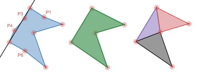
Consider the following example in Figure 1. For the most part it’s a pretty standard shape, but there’s a little piece of it that sticks out. A possible decomposition of the shape is also shown: two shapes, one triangle and one polygon.
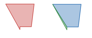
While this is a perfectly valid decomposition, it’s not great for physical simulation. The green triangle is small and thin which can cause this object to behave oddly with other objects. Things like sticking together during collision come to mind.
The question is whether the green bit is even necessary for realistic collision. It might be, but often it’s not, so what happens if we just ignore the green triangle? You could post-process the convex decomposition and remove problem shapes based on area, length, or other criteria, but you run the risk of removing shapes internal to the overall decomposition.
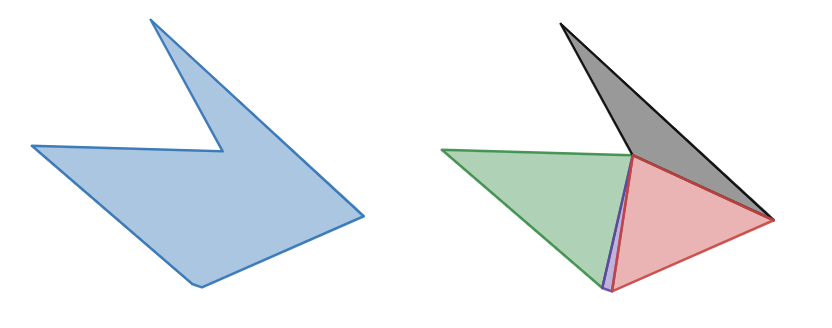
Consider figure 2 of a non-convex polygon that we’ve decomposed. If you simply remove the purple triangle you’ll leave a gap which is probably worse than leaving the problem triangle in. Is the purple triangle providing any tangible benefit to physical simulation? No, it’s just noise. We need a way to pre-process the simple polygon to simplify it further, then decompose it.
NOTE: While this is a poor example of a convex decomposition, it’s a perfectly valid one. Let’s imagine the purple and green shapes were combined, does the additional information of that extra feature provide value to physical simulation? Again, it’ll depend on your use-case, but I’d argue that it has no value and only slows down the simulation.
NOTE: While polygon simplification and convex decomposition are great, it’s no substitute for manually designed collision shapes.
Algorithms
There are a number of algorithms out there to do polygon simplification but I’ll be focusing on three in particular:
- Vertex Cluster Reduction
- Douglas-Peucker
- Visvalingam
All of these attempt to remove insignificant features of an input simple polygon. Consider the input of these algorithms an ordered list of vertices of the simple polygon in clock-wise or counter clock-wise winding.
Vertex Cluster Reduction
By far the simplest algorithm to implement and understand. The basic concept is to remove adjacent vertices that are too close given a minimal distance. The algorithm is \(O(n)\) complexity and can be used as a first pass before employing another algorithm.
1
2
3
4
5
6
7
8
9
10
11
12
13
14
15
16
17
18
19
20
// NOT INTENDED TO BE SOURCE CODE - MORE PSUEDO CODE
List<Vertex> reduce(List<Vertex> vertices, double minDistance) {
    List<Vertex> simplified = new ArrayList<Vertex>;
    int size = vertices.size();

    Vertex ref = vertices.get(0);
    simplified.add(ref);
    for (int i = 1; i < size; i++) {
        Vertex v0 = vertices.get(i);
        if (ref.distance(v0) > minDistance) {
            // set the new reference vertex
            ref = v0;
            // add it to the simplified polygon
            simplified.add(v0);
        }
        // if it's smaller, then we ignore the vertex
        // and continue
    }
    return simplified;
}
If we applied this to our second example above, we’d remove one of the red points and end up with the following simple polygon and it’s respective decomposition:
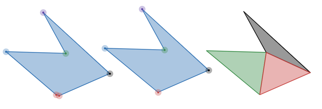
Nice! But the algorithm can’t catch cases like figure 4 where the vertices are not clustered. Vertices P1, P3, P4, and P6 provide little value to the overall structure of the shape. Unfortunately, decomposing this will produce an unnecessary amount of elements. For this we need something more complex.
Douglas-Peucker
The Douglas-Peucker algorithm is a \(O(n log_2 n)\) complexity algorithm that actually operates on polylines instead of polygons, but can be adapted for polygons. The basic concept is to draw a line from one point to another, check the distance to the line for all points in between, if all the points are less than a minimum distance, then remove all those points. If there’s one point that’s more than or equal to the minimum distance, subdivide the polyline into two, and perform the same steps on each one.
1
2
3
4
5
6
7
8
9
10
11
12
13
14
15
16
17
18
19
20
21
22
23
24
25
26
27
28
29
30
31
32
33
34
35
// NOT INTENDED TO BE SOURCE CODE - MORE PSUEDO CODE
List<Vertex> dp(List<Vertex> polyline, double max) {
    int size = polyline.size();
    Vertex first = polyline.get(0);
    Vertex last = polyline.get(size - 1);

    double maxDistance;
    int maxVertex;
    for (int i = 1; i < size - 1; i++) {
        Vertex v = polyline.get(i);
        // get the distance from v to the line created by first/last
        double d = distance(v, first, last);
        if (d > maxDistance) {
            maxDistance = d;
            maxVertex = i;
        }
    }

    if (maxDistance >= max) {
        // subdivide
        List<Vertex> one = dp(polyline.sublist(0, maxVertex + 1));
        List<Vertex> two = dp(polyline.sublist(maxVertex, size));
        // rejoin the two (TODO without repeating the middle point)
        List<Vertex> simplified = new ArrayList<Vertex>();
        simplified.addAll(one);
        simplified.addAll(two);
        return simplified;
    } else {
        // return only the first/last vertices
        List<Vertex> simplified = new ArrayList<Vertex>();
        simplified.add(first);
        simplified.add(last);
        return simplified;
    }
}
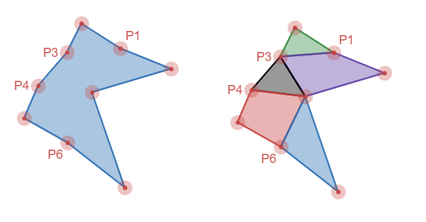
If we run through this process until completion, we end up with vertices P1, P2, P3, and P6 removed - nearly half the verticies. This results in almost half the convex shapes in the decomposition. In addition, the parts that are left are nice and chunky too.
NOTE: The number of vertices reduced will be highly dependent on where the splits are since there’s no re-processing of those vertices where the splits occur. It shouldn’t be a problem since these vertices are the farthest from the line, but it’s possible this could be an issue for the initial split.
The first image is an example of one of the stages of the algorithm where it removed vertices P3 and P4 since they were not sufficiently far from the line between P2 and P5 (not labeled).
Visvalingam
Visvalingam is an alternate \(O(n log_2 n)\) algorithm that takes a similar, but slightly different approach. Instead of computing the distance between the points and a line and recursively subdividing, it looks at the triangular area of each vertex, sorts them, and removes them until the only ones left are above a certain minimum area. For example, using same shape as before, but highlighting all the triangular areas:
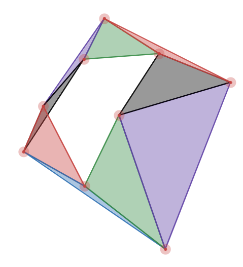
We can see from this picture that the small blue, purple, black, and red areas would clearly be elimitated due to their area, whereas the large green, black, red, and purple areas would remain. The areas are removed by removing the vertex that creates the triangle.
One benefit of this algorithm is that it’s simpler - no subdivision or recombining is necessary nor recursion. The algorithm goes something like this:
1
2
3
4
5
6
7
8
9
10
11
12
13
14
15
16
17
18
19
20
21
22
23
24
25
26
27
28
29
30
31
// NOT INTENDED TO BE SOURCE CODE - MORE PSUEDO CODE
List<Vertex> visvalingam(List<Vertex> vertices, double minArea) {
    // iterate on all input vertices O(n) and compute the area
    // and put them in a priority queue to sort them by area O(log n)
    Queue<VertexWithArea> queue = new PriorityQueue<VertexWithArea>();

    int size = vertices.size();
    for (int i = 0; i < size; i++) {
        Vertex v0 = vertices.get(i == 0 ? size-1 : i-1);
        Vertex v1 = vertices.get(i);
        Vertex v2 = vertices.get(i+1 == size ? 0 : i+1);

        double area = getTriangleArea(v0, v1, v2);
        VertexWithArea vwa = new VertexWithArea(v1, area);
        queue.add(vwa);
    }

    // iterate over the priority queue and eliminate vertices
    do {
        VertexWithArea vwa = queue.poll();
        if (vwa.area < minArea) {
            // remove this vertex

            // NOTE: you need to recompute the area of the adjacent vertices
            // and have them get resorted in the priority queue (just remove them
            // and re-add them back or something)
        }
    } while (!queue.isEmpty());

    // what's left is the simplified polygon
}
This would yield the same result as the Douglas-Peucker algorithm above, but that’s not guaranteed. Another nice attribute of this algorithm is that it’s ever evolving the result, to the point that it could be use for other purposes like zoomable maps.
The downside of this algorithm is the selection of the minimum area. It’s much harder to select that properly than a distance metric.
Self-Intersection
The last topic I want to mention is that of self-intersection. All these algorithms will reduce the simple polygon by removing vertices. The removal of a vertex is not guaranteed to prevent self-intersections in the resulting simplified polygon. For example, figure 7 shows a simple polygon where the smallest triangle (green area) contains another vertex (P5). If we remove P2 (and therefore the green triangle) we’d create a self-intersection - the segment from P1 to P3 would intersect the segments connecting to P5.
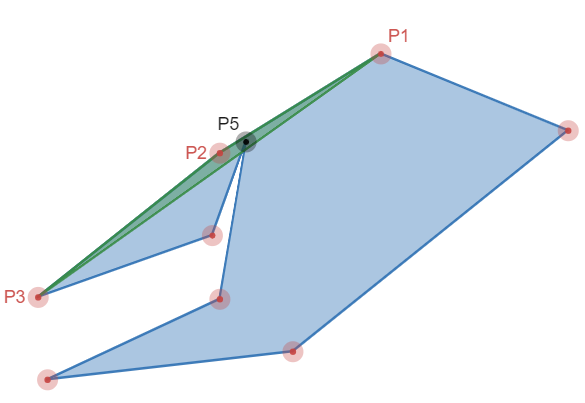
We could handle this in a straight forward way by testing all segments against the segment we’re adding (P1-P3), but that’d be pretty inefficient and take our computational complexity up to \(O(n^2)\). If you squint really hard though, you can probably see that this is just a collision detection problem and we’ve dealt with it before.
Recall that for global collision detection we have a phased approach that starts with a broadphase which eliminates those pairs that cannot intersect, but allows some pairs that may not be intersecting proceed to the next phase. The next phase, the narrowphase, performs the accurate collision detection. We can apply the same concept here, in fact, you could even employ the very same algorithm and implementation. Dump all the individual segments into your broadphase and then everytime you detect a vertex to remove, check the resulting line segment for collisions with the broadphase. Then, check those potential collisions using a simple segment-vs-segment intersection test. You can even stop the whole collision detection process when you detect the first collision. Nice!
We’ve now detected a self-intersection, but what do we do about it? Well, the choice is yours really. I raised the white flag and just left the vertex in the resulting polygon and continued processing other vertices. You could try to generate a new point which removes the feature, but doesn’t create the self-intersection too.
Results
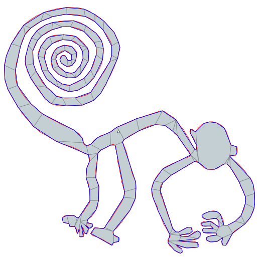
To top things off I’d like to share some results of how well this process can work for complex simple polygons.
| Shape | Original # Vertices | Original # Convex | Simplified # Vertices | Simplified # Convex |
|---|---|---|---|---|
| Nazca Monkey | 1204 | 444 | 304 | 124 |
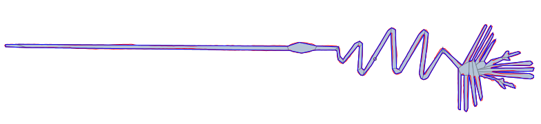
| Nazca Heron | 1036 | 370 | 115 | 43 |
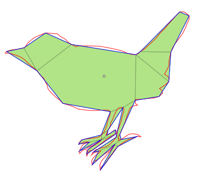
| Bird | 275 | 102 | 38 | 18 |
Final Remarks
In summary, polygon simplification can be used to reduce the complexity of simple polygons to support better decompositions which supports better physical simulation. These algorithms can be used in realtime simulations to cleanse user input, but will modify the input. Choice of the minimum distances/area is the remaining hurdle to using these without user input. One thought I have for that would be to analyze the original simple polygon and come up some metrics to automatically determine the minimum values. Ideally all of this would be part of a toolchain where you can specify these parameters to achieve the most optimal result for your scenario, likely tweaking the result further manually.
References
- Reference implementation for this post
- Vertex Cluster Reduction
- Douglas-Peucker (Wikipedia)
- Douglas-Peucker
- Visvalingam
- Visvalingam with self-intersection avoidance
- Visvalingam Paper
- A source with a lot of information/links on line simplification
- Coastline Paradox
- Fractal Dimensions