Today I’m going to talk about the other collision detection algorithm packaged with the dyn4j project. You can find a lot of GJK documentation but much of it is really technical mostly because they are research papers. I strongly recommend this video tutorial and to be honest you may not even need to read any further after watching. But if you feel you need more information after watching the video please read on.
- Introduction
- Convexity
- Minkowski Sum
- The Simplex
- The Support Function
- Creating The Simplex
- Determining Collision
- Iteration
- Checking The Simplex
Introduction
GJK, like SAT, only operates on convex shapes. One of the more attractive features of GJK is that it can support any shape that implements a “support function” (we’ll talk about this later). Therefore, unlike SAT, you don’t need to handle curved shapes, for example, using special code or algorithms.
GJK is an iterative method but converges very fast and if primed with the last penetration/separation vector can run in near constant time. It’s a better alternative to SAT for 3D environments because of the number of axes that SAT must test.
GJK’s original intent was to determine the distance between two convex shapes. GJK can also be used to return collision information for small penetrations and can be supplemented by other algorithms for deeper penetrations.
Convexity
As I said earlier, GJK is an algorithm that can only be used with convex shapes. See my post on SAT for an explaination of convexity.
Minkowski Sum
The GJK algorithm relies heavily on a concept called the Minkowski Sum. The Minkowski Sum conceptually is very easy to understand. Let’s say you have two shapes, the Minkowski Sum of those shapes is all the points in shape1 added to all the points in shape2:
\[A + B = \{\vec{a} + \vec{b} \: \mid \: \vec{a} \in A, \vec{b} \in B\}\]If both shapes are convex, the resulting shape is convex. You are probably thinking, “Ok, thats great, but how does this relate?” The significance is not in the addition but if we choose to do subtraction instead, things will get more interesting:
\[A - B = \{\vec{a} - \vec{b} \: \mid \: \vec{a} \in A, \vec{b} \in B\}\]As a side note before we continue, even though we are using a “difference” operator this isn’t called the Minkowski Difference. Instead, it’s still called the Minkowski Sum. For the remainder of the article I will refer to this as the Minkowski Difference just for clarity sake.
Moving on, the key with performing a difference operation in the Minkowski Sum is that:
If two shapes are overlapping/intersecting the Minkowski Difference of those shapes will contain the origin.
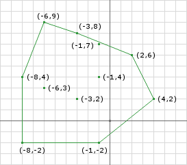
Lets look at an example, take the two shapes in figure 1 and perform the Minkowski Difference on them and you will get the shape in figure 2. Notice that the resulting shape contains the origin. This is because the shapes are intersecting.
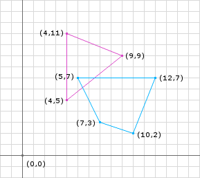
Now performing this operation required shape1.vertices.size * shape2.vertices.size * 2 subtractions. This is significant because a shape is made up of an infinite number of points. Since both shapes are convex and defined by outermost vertices we only need to perform this operation on the vertices. The great thing about GJK is that you don’t actually have to calculate the Minkowski Difference.
The Simplex
We don’t want to compute the Minkowski Difference. Instead we just want to know whether the Minkowski Difference contains the origin or not. If it does, then we know that the shapes are intersecting, if it doesn’t, then they aren’t.
Instead what we can do is iteratively build a polygon inside the Minkowski Difference that attempts to enclose the origin. If the polygon we build contains the origin (and is contained in the Minkowski Difference) then we can say the Minkowski Difference contains the origin. This polygon that we want to build is called the Simplex.
The Support Function
So the next question is how do we build the Simplex? The Simplex is built using whats called a Support Function. The support function should return a point inside the Minkowski Difference given the two shapes. We already know that we can take a point from shape1 and a point from shape2 and subtract them to obtain a point in the Minkowski Difference, but we don’t want it to be the same point every time.
We can ensure that we don’t get the same point every call to the support function if we make the support function dependent on a direction \(\vec{d}\). In other words, if we make the support function return the farthest point in the direction of \(\vec{d}\), we can choose a different direction later to obtain a different point.
Choosing the farthest point in a direction has significance because it creates a simplex who contains a maximum area therefore increasing the chance that the algorithm exits quickly. In addition, we can use the fact that all the points returned this way are on the edge of the Minkowski Difference and therefore if we cannot add a point past the origin along some direction we know that the Minkowski Difference does not contain the origin. This increases the chances of the algorithm exiting quickly in non-intersection cases. More on this later.
1
2
3
4
5
6
7
8
9
10
public Point support(Shape shape1, Shape shape2, Vector d) {
  // d is a vector direction (doesn't have to be normalized)
  // get points on the edge of the shapes in opposite directions
  Point p1 = shape1.getFarthestPointInDirection(d);
  Point p2 = shape2.getFarthestPointInDirection(d.negative());
  // perform the Minkowski Difference
  Point p3 = p1.subtract(p2);
  // p3 is now a point in Minkowski space on the edge of the Minkowski Difference
  return p3;
}
Creating The Simplex
Lets start with an example. Using the shapes in figure 2 and performing the support function 3 times:
First lets start by using \(\vec{d}\) = (1, 0)
1
2
3
p1 = (9, 9)
p2 = (5, 7)
p3 = p1 - p2 = (4, 2)
Next lets use \(\vec{d}\) = (-1, 0)
1
2
3
p1 = (4, 5)
p2 = (12, 7)
p3 = p1 - p2 = (-8, -2)
Notice that p1 could have been (4, 5) or (4, 11). Both will produce a point on the edge of the Minkowski Difference.
Next lets use \(\vec{d}\) = (0, 1)
1
2
3
p1 = (4, 11)
p2 = (10, 2)
p3 = p1 - p2 = (-6, 9)
we obtain the Simplex illustrated in Figure 3.

Determining Collision
We said earlier that we know that the two shapes are intersecting if the simplex in the Minkowski Difference contains the origin. In Figure 3, the Simplex doesn’t contain the origin, but we know that the two shapes are intersecting. The problem here is that our first guess (at choosing directions) didn’t yield a Simplex that enclosed the origin.
If instead I choose \(\vec{d}\) = (0, -1) for the third Minkowski Difference direction:
1
2
3
p1 = (4, 5)
p2 = (5, 7)
p3 = p1 - p2 = (-1, -2)
This yields the simplex shown in figure 4 and now we contain the origin and can determine that there is a collision.
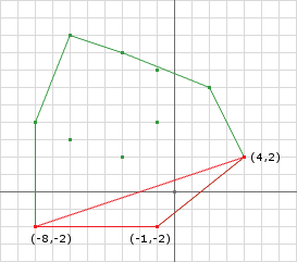
So, as we have seen, the choice of direction can affect the outcome. We can also see that if we obtain a Simplex that does not contain the origin we can calculate another point and use it instead.
This is where the iterative part of the algorithm comes in. We cannot gaurentee that the first 3 points we choose are going to contain the origin nor can we guarentee that the Minkowski Difference contains the origin. We can modify how we choose the points by only choosing points in the direction of the origin. If we change the way we choose the third Minkowski Difference point to below we can enclose the origin.
For the first support point, a, we can choose an arbitrary direction. Now, we want the support point, b, to be in a different direction so that it’s not the same as a. To do that, we simply negate the original direction. Now that we have two support points, a and b, we can use those to form a vector, get the normal of that vector in the direction of the origin, as use that as our new direction to get the last support point, c.
1
2
3
4
5
6
7
d = ...
a = support(..., d)
b = support(..., -d)
AB = b - a
AO = ORIGIN - a
d = (AB x AO) x AB
c = support(..., d)
So now we only need to choose d for the first Minkowksi Difference point. There are a number of options here, an arbitrary direction as stated earlier, the direction created by the difference of the shapes centers, etc. Any will work but some might be better in the case of non-intersection.
NOTE: AB stands for “point A to point B” which is found by taking \(\vec{b} - \vec{a}\) not the other way around. This applies to all instances: AO, AC, etc. for example.
Iteration
Even though we changed the above to determine collision we still may not get a Simplex that contains the origin in those three steps. We must iteratively create the Simplex such that the Simplex is getting closer to containing the origin. We also need to check for two conditions along the way: 1) does the current simplex contain the origin? and 2) are we able to enclose the origin?
Lets look at the skeleton of the iterative algorithm:
1
2
3
4
5
6
7
8
9
10
11
12
13
14
15
16
17
18
19
20
21
22
23
24
25
26
27
28
29
Vector d = // choose a search direction
// get the first Minkowski Difference point
Simplex.add(support(A, B, d));
// negate d for the next point
d.negate();
// start looping
while (true) {
  // add a new point to the simplex because we haven't terminated yet
  Simplex.add(support(A, B, d));
  // make sure that the last point we added actually passed the origin
  if (Simplex.getLast().dot(d) <= 0) {
    // if the point added last was not past the origin in the direction of d
    // then the Minkowski Sum cannot possibly contain the origin since
    // the last point added is on the edge of the Minkowski Difference
    return false;
  } else {
    // otherwise we need to determine if the origin is in
    // the current simplex
    if (Simplex.contains(ORIGIN)) {
      // if it does then we know there is a collision
      return true;
    } else {
      // otherwise we cannot be certain so find the edge who is
      // closest to the origin and use its normal (in the direction
      // of the origin) as the new d and continue the loop
      d = getDirection(Simplex);
    }
  }
}
Next lets use the skeleton with our example in Figure 1. Lets set our initial direction to the vector from the center of shape1 to the center of shape2:
1
2
3
4
d = c2 - c1 = (9, 5) - (5.5, 8.5) = (3.5, -3.5) = (1, -1);
p1 = support(A, B, d) = (9, 9) - (5, 7) = (4, 2);
Simplex.add(p1);
d.negate() = (-1, 1);
Then we start the loop:
Iteration 1
Note that the following triple product expansion is used: \((\vec{a} \times \vec{b}) \times \vec{c} = \vec{b}(\vec{c} \cdot \vec{a}) - \vec{a}(\vec{c} \cdot \vec{b})\) to evaluate the triple product.
1
2
3
4
5
6
7
8
9
10
11
last = support(A, B, d) = (4, 11) - (10, 2) = (-6, 9);
proj = (-6, 9).dot(-1, 1) = 6 + 9 = 15
// we past the origin so check if we contain the origin
// we dont because we are line
// get the new direction by (AB x AO) x AB
AB = (-6, 9) - (4, 2)  = (-10, 7);
AO = (0, 0) - (-6, 9) = (6, -9);
(AB x AO) x AB = AO(149) - AB(-123)
               = (894, -1341) - (1230, -861)
               = (-336, -480)
               = (-0.573, -0.819)
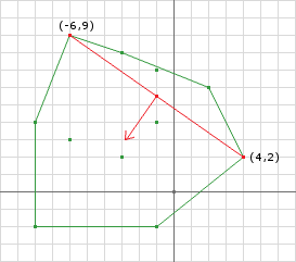
Figure 5 shows the resulting simplex after iteration 1. We have a line segment (brown) simplex with the next direction (blue) pointing perpendicular to the line towards the origin. One note, the direction does not need to be normalized (see iteration 2) but I’m doing it here so we can verify the direction given our scale.
Iteration 2
1
2
3
4
5
6
7
8
9
10
11
12
last = support(A, B, d) = (4, 5) - (12, 7) = (-8, -2)
proj = (-8, -2).dot(-336, -480) = 2688 + 960 = 3648
// we past the origin so check if we contain the origin
// we dont (see Figure 6a)
// the new direction will be the perp of (4, 2) and (-8, -2)
// and the point (-6, 9) can be removed
AB = (-8, -2) - (4, 2)  = (-12, -4);
AO = (0, 0) - (-8, -2) = (8, 2);
(AB x AO) x AB = AO(160) - AB(-104)
               = (1280, 320) - (1248, 416)
               = (32, -96)
               = (0.316, -0.948)
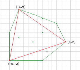
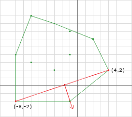
After the second iteration we have not enclosed the origin yet but still cannot conclude that the shapes are not intersecting. In the second iteration we removed the (-6, 9) point because all we need is 3 points at any time and we add a new point at the beginning of every iteration.
Iteration 3
1
2
3
4
last = support(A, B, d) = (4, 5) - (5, 7) = (-1, -2)
proj = (-1, -2).dot(32, -96) = -32 + 192 = 160
// we past the origin so check if we contain the origin
// we do (Figure 7)!

Checking The Simplex
We have glazed over two operations in the algorithm, using just pictures and inspection. One is, how do we know that the current simplex contains the origin? The other being, how do we choose the next direction? In the pseudo code above I made these operations separate for the sake of clarity, but in reality they really should be together since they need to know much of the same information.
We can determine where the origin lies with respect to the simplex by performing a series of plane tests (line tests for 2D) where each test consists of simple dot products. The first case that must be handled is the line segment case. So lets look at the first iteration from the example above. After adding the second point on line 9, the simplex is now a line segment. We can determine if the simplex contains the origin by examining the Voronoi regions (see Figure 8).
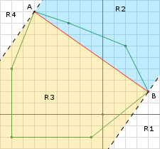
The line segment is defined as A to B where A is the last point added to the simplex. We know that both A and B are on the edge of the Minkowski Difference and therefore the origin cannot lie in R1 or R4. We can make this assumption because the check from line 11 returned false indicating that we passed the origin when we obtained our next point. The origin can only lie in either R2 or R3 and since a line segment cannot contain the origin then all that needs to be done is to select a new direction. This can be done, as previously stated, by using the perp of AB in the direction of the origin:
1
2
3
4
// the perp of AB in the direction of O can be found by
AB = B - A;
AO = O - A;
perp = (AB x AO) x AB;
The catch here is what happens when O lies on the line? If that happens the perp will be a zero vector and will cause the check on line 11 to fail. This can happen in two places: 1) inside the Minkowski Sum and 2) on the edge of the Minkowski Sum. The latter case indicates a touching contact rather than penetration so you will need to make a decision on whether this is considered a collision or not. In either case, you can use either the left or right hand normal of AB as the new direction.
Now lets examine the second iteration. The second iteration turns our simplex into a triangle (Figure 9).
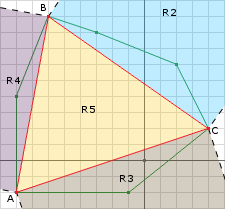
The white regions do not have to be tested since the origin cannot be past any of those points since each point was added because they passed the check on line 11. R2 cannot contain the origin because the last direction we choose was in the opposite direction. So the only regions to test are R3, R4, and R5. We can perform (AC x AB) x AB to yield the perpendicular vector to AB. Then we perform: ABPerp.dot(AO) to determine if the origin is in region R4.
1
2
3
4
5
6
7
8
9
10
11
AB = (-6, 9) - (-8, -2) = (2, 11)
AC = (4, 2) - (-8, -2) = (12, 4)
// (AC x AB) x AB = AB(AB.dot(AC)) - AC(AB.dot(AB))
ABPerp = AB(68) - AC(125)
       = (136, 748) - (1500, 500)
       = (-1364, 248)
       = (-11, 2)
// compute AO
AO = (0, 0) - (-8, -2) = (8, 2)
ABPerp.dot(AO) = -11 * 8 + 2 * 2 = -84
// its negative so the origin does not lie in R4
So with one more test we can determine where the origin lies:
1
2
3
4
5
6
7
8
9
10
11
AB = (-6, 9) - (-8, -2) = (2, 11)
AC = (4, 2) - (-8, -2) = (12, 4)
// (AB x AC) x AC = AC(AC.dot(AB)) - AB(AC.dot(AC))
ACPerp = AC(68) - AB(160)
       = (816, 272) - (320, 1760)
       = (496, -1488)
       = (1, -3)
// compute AO
AO = (0, 0) - (-8, -2) = (8, 2)
ACPerp.dot(AO) = 1 * 8 + -3 * 2 = 2
// its positive so that means the origin lies in R3
So we have found that the origin lies in R3 so now we need to select a direction so that we get our next Minkowski Difference point in that direction. This is easy since we know that AC was the line segment whose Voronoi region the origin was contained in:
1
(AC x AO) x AC
And since we are using points A and C we can get rid of B since we didn’t use it. The new code becomes:
1
2
3
4
5
6
7
8
9
10
11
12
13
14
15
16
17
18
19
20
21
22
23
24
25
26
27
28
29
30
31
32
33
34
35
36
37
38
39
40
41
42
43
44
45
46
47
48
49
50
51
52
53
54
55
56
57
58
59
60
61
62
63
64
65
66
67
68
69
70
71
Vector d = // choose a search direction
// get the first Minkowski Difference point
Simplex.add(support(A, B, d));
// negate d for the next point
d.negate();
// start looping
while (true) {
  // add a new point to the simplex because we haven't terminated yet
  Simplex.add(support(A, B, d));
  // make sure that the last point we added actually passed the origin
  if (Simplex.getLast().dot(d) <= 0) {
    // if the point added last was not past the origin in the direction of d
    // then the Minkowski Sum cannot possibly contain the origin since
    // the last point added is on the edge of the Minkowski Difference
    return false;
  } else {
    // otherwise we need to determine if the origin is in
    // the current simplex
    if (containsOrigin(Simplex, d) {
      // if it does then we know there is a collision
      return true;
    }
  }
}

public boolean containsOrigin(Simplex s, Vector d) {
  // get the last point added to the simplex
  a = Simplex.getLast();
  // compute AO (same thing as -A)
  ao = a.negate();
  if (Simplex.points.size() == 3) {
    // then its the triangle case
    // get b and c
    b = Simplex.getB();
    c = Simplex.getC();
    // compute the edges
    ab = b - a;
    ac = c - a;
    // compute the normals
    abPerp = tripleProduct(ac, ab, ab);
    acPerp = tripleProduct(ab, ac, ac);
    // is the origin in R4
    if (abPerp.dot(ao) > 0) {
      // remove point c
      Simplex.remove(c);
      // set the new direction to abPerp
      d.set(abPerp);
    } else {
      // is the origin in R3
      if (acPerp.dot(ao) > 0) {
        // remove point b
        Simplex.remove(b);
        // set the new direction to acPerp
        d.set(acPerp);
      } else{
        // otherwise we know its in R5 so we can return true
        return true;
      }
    }
  } else {
    // then its the line segment case
    b = Simplex.getB();
    // compute AB
    ab = b - a;
    // get the perp to AB in the direction of the origin
    abPerp = tripleProduct(ab, ao, ab);
    // set the direction to abPerp
    d.set(abPerp);
  }
  return false;
}
This completes the tutorial for the GJK collision detection algorithm. The original GJK algorithm computed a distance between the two convex shapes. I plan to cover this portion of the algorithm in another post since this post is already way too long. Also, as I said earlier, if you need collision information (normal and depth) you will need to modify the GJK algorithm or supplement it with another algorithm. EPA is one supplement algorithm which I plan to cover in another post. Until next time…


Why is shape1.vertices.size * shape2.vertices.size * 2 subtractions?
I feel shape1.vertices.size * shape2.vertices.size is enough.