The last installment talked about the GJK algorithm as it pertains to collision detection. The original algorithm actually is used to obtain the distance and closest points between two convex shapes.
Introduction
The algorithm uses much of the same concepts to determine the distance between the shapes. The algorithm is iterative, uses the Minkowski Sum/Difference, looks for the origin, and uses the same support function.
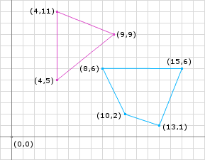
Overview
We know that if the shapes are not colliding that the Minkowski Difference will not contain the origin. Therefore instead of iteratively trying to enclose the origin with the simplex, we will want to generate a simplex that is closest to the origin. The closest simplex will always be on the edge of the Minkowski Difference. The closest simplex for 2D could be either a single point or a line.
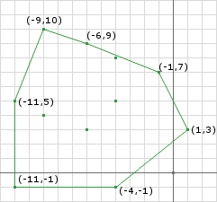
Minkowski Sum
Just as we did for the collision detection portion of GJK in the previous post, the algorithm also needs to know the Minkowski Sum (Difference is what I will call it, see the GJK post).
Taking the same shapes from the GJK post and separating them (Figure 1) yeilds the same Minkowski Difference only translated slightly (Figure 2). We notice that the origin is not contained within the Minkowski Difference, therefore there is not a collision.
The Distance
The distance can be calculated by finding the closest point on the Minkowski Difference to the origin. The distance is then the magnitude of the closest point. By inspection, we see that the edge created by the points (-4, -1) and (1, 3) is the closest feature to the origin. Naturally the closest point to the origin is the point on this edge that forms a right angle to the origin. We can calculate the point by:
1
2
3
4
5
6
7
8
9
10
11
12
13
14
15
16
A = (-4, -1)
B = (1, 3)
// create the line
AB = (1, 3) - (-4, -1) = (5, 4)
AO = (0, 0) - (-4, -1) = (4, 1)
// project AO onto AB
AO.dot(AB) = 4 * 5 + 1 * 4 = 24
// get the length squared
AB.dot(AB) = 5 * 5 + 4 * 4 = 41
// calculate the distance along AB
t = 24 / 41
// calculate the point
AB.mult(t).add(A) = (120 / 41, 96 / 41) + (-4, -1)
                  = (-44 / 41, 55 / 41)
                  = (-1.07, 1.34)
d = (-1.07, 1.34).magnitude() = 1.71
This is a simple calculation since we know what points of the Minkowski Difference to use.
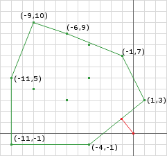
Iteration
Like the collision detection routine of GJK the distance routine is iterative (and almost identical for that matter). We need to iteratively build a simplex which contains the closest points on the Minkowski Difference to the origin. The points will be obtained using a similar method of choosing a direction, using the support function, and checking for the termination case.
Lets examine some psuedo code:
1
2
3
4
5
6
7
8
9
10
11
12
13
14
15
16
17
18
19
20
21
22
23
24
25
26
27
28
29
30
31
32
33
34
35
36
37
38
39
40
41
42
43
44
45
46
47
48
49
50
51
52
53
54
55
56
57
58
59
60
61
62
63
64
65
66
67
68
// exactly like the previous post, use whatever
// initial direction you want, some are more optimal
d = // choose a direction
// obtain the first Minkowski Difference point using
// the direction and the support function
Simplex.add(support(A, B, d));
// like the previous post just negate the
// the prevous direction to get the next point
Simplex.add(support(A, B, -d));
// obtain the point on the current simplex closest
// to the origin (see above example)
// start the loop
d = ClosestPointToOrigin(Simplex.a, Simplex.b);
while (true) {
  // the direction we get from the closest point is pointing
  // from the origin to the closest point, we need to reverse
  // it so that it points towards the origin
  d.negate();
  // check if d is the zero vector
  if (d.isZero()) {
    // then the origin is on the Minkowski Difference
    // I consider this touching/collision
    return false;
  }
  // obtain a new Minkowski Difference point along
  // the new direction
  c = support(A, B, d);
  // is the point we obtained making progress
  // towards the goal (to get the closest points
  // to the origin)
  double dc = c.dot(d);
  // you can use a or b here it doesn't matter
  // since they will be equally distant from
  // the origin
  double da = Simplex.a.dot(d);
  // tolerance is how accurate you want to be
  if (dc - da < tolerance) {
    // if we haven't made enough progress,
    // given some tolerance, to the origin,
    // then we can assume that we are done

    // NOTE: to get the correct distance we
    // need to normalize d then dot it with
    // a or c
    // OR since we know that d is the closest
    // point to the origin, we can just get
    // its magnitude
    distance = d.magnitude();
    return true;
  }
  // if we are still getting closer then only keep
  // the points in the simplex that are closest to
  // the origin (we already know that c is closer
  // than both a and b so we only need to choose
  // between these two)
  p1 = ClosestPointToOrigin(Simplex.a, c);
  p2 = ClosestPointToOrigin(c, Simplex.b);
  // getting the closest point on the edges AC and
  // CB allows us to compare the distance between
  // the origin and edge and choose the closer one
  if (p1.magnitude() < p2.magnitude()) {
    Simplex.b = c;
    d = p1;
  } else {
    Simplex.a = c;
    d = p2;
  }
}
The first few lines look a lot like the previous GJK post. The difference is the building of our simplex. We are using the same idea of a simplex, we use the same support function and roughly the same logic, however, we only keep 2 points at all times (3D would be 3 points) and we find a point on the simplex closest to the origin instead of finding the Voronoi region that the origin lies in.
As we did in the previous post this is best explained by running through an example. Let’s take the example above from Figure 1 and run through the iterations.
Pre Iteration:
1
2
3
4
5
6
7
8
9
// im going to choose the vector joining the
// centers of the objects as the initial d
d = (11.5, 4.0) - (5.5, 8.5) = (6, -4.5)
Simplex.add(support(A, B, d)) = (9, 9) - (8, 6) = (1, 3)
Simplex.add(support(A, B, -d)) = (4, 11) - (13, 1) = (-9, 10)
// calculate new d (for brevity, we'll just look at figure 4)
d = (1, 3) // then negate
d = (-1, -3)
// start the iterations</pre>
Iteration 1:
1
2
3
4
5
6
7
8
9
10
11
// get a new point in this direction
c = support(A, B, d) = (4, 5) - (15, 6) = (-11, -1)
// are we still moving closer to the origin?
dc = 11 + 3 = 14
da = -1 - 9 = -10
// 14 - -10 = 24 not small enough
// by inspection, edge AC [(1, 3) to (-11, -1)] is closer than BC [(-9, 10) to (-11, -1)]
// so keep a and replace b with c
b = c
// use p1 as the next direction
d = p1
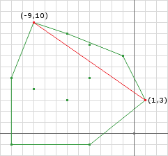
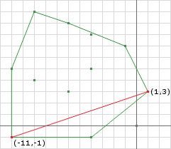
In this first iteration I didn’t go through the trouble of calculating p because its obviously going to be the end point a. If you performed the real calculation, like the code will do, you will obtain the same result. We notice that even though the closest point is a point already on the simplex, we can still use it as the next direction. We obtain a new point using the new direction and keep the two closest points.
Iteration 2:
1
2
3
4
5
6
7
8
9
10
11
12
d = (0.8, -2.4)
// get a new point in this direction
c = support(A, B, d) = (4, 5) - (8, 6) = (-4, -1)
// are we still moving closer to the origin?
dc = -3.2 + 2.4 = -0.8
da = 0.8 - 7.2 = -6.4
// -0.8 - -6.4 = 5.6 not small enough
// by inspection, edge AC [(1, 3) to (-4, -1)] is closer than BC [(-11, -1) to (-4, -1)]
// so keep a and replace b with c
b = c
// use p1 as the next direction
d = p1
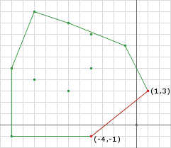
Notice that our simplex is getting closer to the origin.
Iteration 3:
Notice in iteration 3 that d is the closest point to the origin and is the same point we found in the Distance section above.
1
2
3
4
5
6
7
8
9
10
d = (1.07, -1.34)
// get a new point in this direction
c = support(A, B, d) = (9, 9) - (8, 6) = (1, 3)
// are we still moving closer to the origin?
dc = -1.07 + 4.02 = 2.95
da = -1.07 + 4.02 = 2.95
// 2.95 - 2.95 = 0 i think thats small enough!
// ||d|| = 1.7147886...
// we done!
distance = 1.71
We notice that when we terminated the difference in projections was zero. This can only happen with two polygons. If either A or B was a shape with a curved edge the difference in projections would approach zero but not obtain zero. Therefore we use a tolerance to handle curved shapes since the tolerance will also work for polygons.
Another problem curved shapes introduce is that if the chosen tolerance is not large enough the algorithm will never terminate. In this case we add a maximum iterations termination case.
One more problem that this algorithm can run into is if the shapes are actually intersecting. If they are intersecting the algorithm will never terminiate. This isn’t as big of a problem since most of the time you will determine if the shapes are colliding first anyway. If not, then we must add a check in the while loop for the simplex containing the origin. This can be done by a simple point in triangle test (2D).
Closest Points
In addition to the distance between the two shapes, we can also determine the closest points on the shapes. To do this we need to store additional information as we progress through the algorithm. If we store the points on the shapes that were used to create the Minkowski Difference points we can use them later to determine the closest points.
For instance, we terminated above with the Minkowski Difference points A = (1, 3) and B = (-4, -1). These points were created by the following points on their respective shapes:
Shape Points
| S1 | S2 | Minkowski Point | |
|---|---|---|---|
| a | (9, 9) | (8,6) | = (1, 3) |
| b | (4, 5) | (8,6) | = (-4, -1) |
The points used to create the Minkowski Difference points are not necessarily the closest points. However, using these source points we can calculate the closest points.
Convex Composition
We see that the points from A and B are not the correct closests points. By inspection we can see that the closest point on B is (8, 6) and the closest point on A is roughly (6.75, 7.25). We must do some calculation to obtain the closest points. Here’ where the definition of a Convex Combination comes in:
\[\begin{align} CC(S) &= \sum_{i=1..n} \lambda_i\vec{p}_i = \lambda_1\vec{p}_1 + ... + \lambda_n\vec{p}_n \:\textrm{where}\: \vec{p}_i \in S \:\textrm{and}\: \lambda_i \in \mathbb{R} \\ \sum_{i=1..n} \lambda_i &= 1 \:\textrm{where}\: \lambda_i >= 0 \end{align}\]We can guarantee that the points we attempt to find will be on the simplex since all convex combinations are within the convex hull of the set \(S\). Any positive values for the \(\lambda\) coefficients ensure we don’t overstep the bounds of the simplex. Our 2D example looks like this:
\[CC(S) = \lambda_1\vec{p}_1 + \lambda_2\vec{p}_2\]Next, let’s say that \(\vec{q}\) is the closest point to the origin on the termination simplex, then we know that the vector from \(\vec{q}\) to the origin must be perpendicular to the line segment \(\vec{l}\) that \(\vec{q}\) lies on. We also know that \(\vec{q}\), because it lies on the edge of the simplex it can be defined as a convex combination of the points \(\vec{a}, \vec{b}\) that make up the line segment \(\vec{l}\).
\[\begin{align} \vec{q} \cdot \vec{l} &= 0 \\ (\lambda_1\vec{a} + \lambda_2\vec{b}) \cdot \vec{l} &= 0 \end{align}\]We need to solve for \(\lambda_1\) and \(\lambda_2\), but to do so we need 2 equations. The second equation comes from the other part of the definition of a convex combination:
\[\begin{align} \sum_{i=1..n} \lambda_i &= 1 \:\textrm{where}\: \lambda_i >= 0 \\ \lambda_1 + \lambda_2 &= 1 \end{align}\]Solving the system of equations we obtain:
\[\begin{align} \lambda_1 + \lambda_2 &= 1 \\ \lambda_1 &= 1 - \lambda_2 \\ \\ (\lambda_1\vec{a} + \lambda_2\vec{b}) \cdot \vec{l} &= 0 \\ ((1 - \lambda_2)\vec{a} + \lambda_2\vec{b}) \cdot \vec{l} &= 0 \\ (\vec{a} - \lambda_2\vec{a} + \lambda_2\vec{b}) \cdot \vec{l} &= 0 \\ (\vec{a} + \lambda_2(\vec{b} - \vec{a})) \cdot \vec{l} &= 0 \\ \vec{a} \cdot \vec{l} + \lambda_2\vec{l} \cdot \vec{l} &= 0 \\ \lambda_2\vec{l} \cdot \vec{l} &= -\vec{a} \cdot \vec{l} \\ \lambda_2 &= -\frac{\vec{a} \cdot \vec{l}}{\vec{l} \cdot \vec{l}} \end{align}\]If we perform this computation on our example above, we get:
1
2
3
4
5
l = (-4, -1) - (1, 3) = (-5, -4)
ldotl = 25 + 16 = 41
ldota = -5 - 12 = -17
lambda2 = 17/41
lambda1 = 24/41
After computing \(\lambda_2\) and \(\lambda_1\) we can compute the closest points by using the definition of the convex combination again, but using the points that made up the Minkowski Difference points (remember that s1 and s2 of A and B were listed in the table above):
1
2
3
4
aClosest = lambda1 * As1 + lambda2 * Bs1
bClosest = lambda1 * As2 + lambda2 * Bs2
aClosest = 24/41 * (9, 9) + 17/41 * (4, 5) = (6.93, 7.34)
bClosest = 24/41 * (8, 6) + 17/41 * (8, 6) = (8, 6)
As we can see we computed the closest points!
There are a couple of problems here we must resolve however.
First, if the Minkowski Difference points \(\vec{a}\) and \(\vec{b}\) are the same point, then \(\vec{l}\) will be the zero vector. This means that later when we divide by the magnitude of \(\vec{l}\) we’ll divide by zero: not good. What this means is that the closest point to the origin is not on a edge of the Minkowski Difference but is a point. Because of this, the support points that made both \(\vec{a}\) and \(\vec{b}\) are the same, and therefore you can just return the support points of \(\vec{a}\) or \(\vec{b}\):
1
2
3
4
if (l.isZero()) {
  aClosest = a.s1;
  bClosest = a.s2;
}
The second problem comes in when either \(\lambda_1\) or \(\lambda_2\) is negative. According to the definition of a convex hull, \(\lambda\) must be greater than zero. If \(\lambda\) is negative, this tells us that the support points of the other Minkowski Difference point are the closest points:
1
2
3
4
5
6
7
if (lambda1 < 0) {
  aClosest = b.s1;
  bClosest = b.s2;
} else if (lambda2 < 0) {
  aClosest = a.s1;
  bClosest = a.s2;
}
Although your tuturial was very helpful and easy to follow, I found some issues:
– On the first iteration, you picked ‘p’ as (1, 3), when the
calculation yelds (1.7, 2.51).
– In the situation shown on fig1.jpg the minkowski difference (blue dots)
doesn’t contain the origin(white dot), but still, the closestPointToOrigin()
routine returns (0,0);
To fix that, before the return i put the following statements:
if the found point is between a and b
return it
else if a.magnitude() < b.magnitude()
return a
else
return b
And the result is fig2.jpg, note that p is the same as a.
F.Y.I: the squares are 20×20 pixels.
Could you give me a opinion about that?
Thank you!
–
fig1.jpg : http://img210.imageshack.us/i/fig1k.jpg/
fig2.jpg : http://img195.imageshack.us/i/fig2ih.jpg/